VAST 2010 MeshLab Tutorial

At VAST 2010 the 11^th  International Symposium on Virtual Reality, Archaeology and Cultural Heritage. (Louvre, Paris, 21-24 Sept. 2010) there will be a full day tutorial of MeshLab.

It will be held by Marco Callieri and Guido Ranzuglia and will cover almost everything of MeshLab, from basic navigation hint to advanced remeshing, measuring and processing tasks. Obviously with a bit of Cultural Heritage pepper here and there.

Target Audience

• People interested in a simple but powerful opensource tool for mesh processing.
• People who need to visualize, edit and convert 3D models.
• People who need small editing, batch process and mesh cleaning.
• People trying to integrate/replace an existing mesh processing pipeline.
• People interested in advanced, custom measuring/processing of 3D models, exploiting state-of-the-art algorithms.

Participants will be given the latest build of the tool plus some test dataset to experiment with the presented features. Bring your own laptop!

RSVP at the FaceBook Event Page

Remeshing and Texturing (1)

In the pipeline of processing 3D data, after you have aligned and merged your range maps, you ofter require to get a nice clean textured mesh. In the last release of MeshLab we included our state-of-the-art parametrization/remeshing algorithm based on abstract parametrization. Now some a two-part tutorial on his practical usage.
Let's start from a medium complexity mesh of a skull (kindly provided and scanned for the VCG Lab by Marco Callieri). You can see it depicted in the two small figures on the right.
The mesh of the skull is composed by 1.000.000 triangles, it has a meaningful per-vertex color (recovered from a set of photos) and, as it often happens, it is topologically dirty.
First of all it is non 2-manifold (there are 7 edges where more than two face are incident) than there are many small holes and handles that make difficult any kind of parametrization.

So the first step is to build a watertight, coarser but topologically sound model.  Poisson surface reconstruction is a perfect filter for this task. A reconstruction at depth 9 is usually good, that generates a mesh of 1.3M of faces.  For this kind of processing a quite faithful geometric representation is not needed, but it is strongly needed that the overall topology is the right one. In this case some portions of the skull are remarkably thin and at low resolutions the poisson surface reconstruction can create unwanted holes. 

After that a further simplification step is needed to bring the model size to a number reasonable for the Isoparametrization engine.  Remember that the when building an abstract parametrization you do not need the full accuracy model but just a model that shares the overall shape and the same topology. For the purpose of the parametrization small details have a very small influence on the overall quality of the parametrization. Side figure depict the watertight Poisson reconstructed surface, note how the nostril cavity was filled (as expected because it was a hole with boundary).

So simplify it our watertight skull up to 50000 triangles. Take care to check Normal Preservation and Topology preservation Flag. The second one is particularly important, infact the basic edge collapse simplification algorithms can during simplification change the topology of the mesh, and while this is usually a nice feature (it allows for example the closure of very small holes) when you start from a mesh that is surely clean (a 2-manifold watertight model) it is better to be sure that such properties are preserved.

After that you can start with creating the Abstract Isoparametrization, a technique we introduced in:


Nico Pietroni, Marco Tarini, Paolo Cignoni
Almost isometric mesh parameterization through abstract domains
IEEE Transaction on Visualization and Computer Graphics, Volume 16, Number 4, page 621-635 - July/August 2010

Without going into details, that you will find in the above paper, the main idea is rather simple. Usually textures are defined in a dominion that is just the (0,0)-(1,1) square on the plane. In our approach as a domain of the parametrization we use a different 2-dimensional domain, the surface of a very coarse simplicial complex that has the same topology of the original mesh and it is composed by just a few hundred triangles. Such an approach is interesting because this abstract parametrization can be used for a number of things, like for example remeshing, texturing, tangent space smoothing etc.

To build the abstract isoparametrization just start the corresponding filter called "Isoparametrization", (default params are ok, you can lower convergence precision to a '1' to speedup a bit and try to change a bit the targeted size of the abstract domain). It is a bit slow so wait some minutes for the processing. At the end of the process, you do not see anything directly but the structure is attached to the mesh and you can use it in the other filters. If you want re-use it for a later use you have to save both the processed mesh and as a separate step the isoparametrization using the "Isoparametrization Save Abstract Domain Filter".

The created isoparametrization can be used to build a standard parametrization over any mesh that is reasonably close to the original one.
In our example we take a simplified version of the original mesh, composed by just 10000 triangles ("Skull_10k.ply"). We transfer over this simplifed mesh the just build isoparametrization
and then using the filter "Iso Parametrization transfer between meshes", setting as source mesh the one with the abstract parametrization (skull_60k_isoparam.ply) and skull_10k.ply as target.

Now we can transform the transferred isoparametrization into a standard atlased parametrization using the "Isoparametrization Build Atlased Mesh" filter. The two image on the right seems equal but you can see that in the lower one the triangles of the mesh have been cut along the triangles of the abstract parametrization in order to get proper atlas regions. At this point your mesh has a standard texture parametrization and it is ready for use it for a variety of operation.

The First thing that we can do is just to transfer the color of the original 1M vertexes color onto a texture according this parametrization. This can be done by using the filter "Transfer color to texture (between 2 meshes)", choose a reasonable texture size (2048x2048 is good) and you will obtain a simplified textured mesh that looks strikingly similar to the original heavy 1M tri model (try to compare the first and last snapshots).

 Summarized Recipe

1. take a 1M tri colored model
2. make the model watertight using Poisson
3. Simplify it to a 50k model (preserving topology)
4. Build the Isoparametrization
5. build another very simple 10k model from the original 1M model
6. transfer the isoparametrization over the very simple model
7. convert the isoparametrization into a standard atlased texture
8. generate a texture with the color from the original 1M model

Next part of the tutorial with remeshing and other hints in a few days...

First MeshLab 1.3.0 beta out!

The first Beta version of MeshLab 1.3.0 is out. A lot of work has been done under the hood and many new features have been added. In the followings some of the notable improvements:

• Totally restructured view/window mechanism. Now you can have:
  
  
  
  • multiple views of the same mesh. 
  • standard orthographic viewing directions (up/down etc)
  • copy/paste of current viewing parameters (you can even save them for later re-use...);
• The Isoparametrization works. Really! A detailed tutorial on how to practically use it will appear in a day or two!
• new Radiance Scaling rendering mode, (thanks to Romain Vergne, Romain Pacanowski, Pascal Barla, Xavier Granier and Christophe Schlick for providing the code and to Gaël Guennebaud for helping out!). More on this new rendering mode on another post, as it deserves more space, for now just look at the side image...

MeshLab on Facebook

Just a short shameless plug to the MeshLab page on facebook (thanks to Marco Callieri who had the idea and set up the page!). Yet another place for disseminating news and bits on MeshLab (like the MeshLab tutorial at the forthcoming ArcheoFoss workshop in Foggia).

Still on the social side I have been happy to discover that the old-style, web 1.0, IRC channel #meshlab on freenode.net is still alive and kicking, with a few generous developers hanging on it...

Assessing open source software as a scholarly contribution

A post that is not strictly related to Computer Graphics, 3D or Cultural Heritage.
Just a small note/rant to point out a recent paper:

Lou Hafer and Arthur E. Kirkpatrick
"Assessing open source software as a scholarly contribution"
Communications of the ACM, Volume 52 ,  Issue 12  (December 2009)

It is an interesting discussion on the fact that "Academic computer science has an odd relationship with software: Publishing papers about software is considered a distinctly stronger contribution than publishing the software".
 
Being a senior researcher before being the lead developer of MeshLab, I have to say that I totally agree with those feelings. I have often thought that devoting a significant portion of my time to the MeshLab project is not a 100% wise move from a career point of view; probably writing a bunch of easy minor-variation papers is much more rewarding and is evaluated better when running for higher positions.


The sad thing is that there are people thinking that the citations coming from the paper you have written about your software are more than enough to reward you for your effort of writing it. Usually these considerations came from computer scientists who do not have perfectly clear what means writing and maintaining real software tools.
Some bare facts:

1. If you write and maintain significant software tools/library then you are serving the research community in a way that is more significant that writing a paper.
2. The time required to develop and maintain sw tools is much larger than the time required to write one paper.
3. Assessing the importance/significance of software is more difficult than assessing the value of papers, no common bibliometric tools (obviously download count is not a good metric).
4. Commissions evaluating people careers usually ignore sw and concentrate on other, more standard, research products (papers, editorial boards, commitee, teaching, prizes, etc).

As a simple consequence, of 2,3,4 and despite of 1, with current career evaluation habits, developing and maintaining sw tools that are significantly useful for the research community is NOT a career maximizing move. And this is, in my humble opinion, definitely, completely, utterly WRONG.

Now when you stumble upon a discontinued piece of code that you would have loved to have maintained, you have an hint of why the original author abandoned it.

Mean Curvature, Cavity Map, ZBrush and nice tricks for enhancing surface shading

There are many many techniques for enhancing the look of a surface by mean of smart shaders. Without touching Non photo-realistic rendering techniques there are many tricks that can helps the perception of the features and the fine details of the surface of an object. ZBrush has popularized one of these techniques with the name of cavity mapping. The main idea is that you detect 'pits' on the surface and you make them of a different color and, very important, very dull. In practice it simulates in a rough way all those materials where in low accessibility regions dust/rust/oxide accumulates while in the most exposed parts the use make them shiny. You can do such effects in MeshLab and they can be very useful for making quick nice renderings of scanned objects; let make a
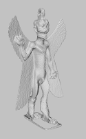
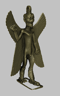
a practical example using a 3D scanned model of ancient statuette of the Assyrian demon Pazuzu (courtesy of Denis Pitzalis C2RMF/Louvre). The plain model (shown on the right) is rather dull and not very readable and at a first glance you cannot appreciate the scale of the scanned details.

You can improve it a bit by adding a bit of ambient occlusion. In MeshLab you can do it in a couple of ways, either computing an actual ambient occlusion term (e.g. a steradian denoting the portion of sky that you can see from a given point) for each vertex (Filter->Color->Vertex ambient occlusion) or just resort to a quick and dirty Screen Space Ambient Occlusion (SSAO) approximation (render->Screen Space Ambient Occlusion).In the first case as a bonus you are able to tweak the computed value as you want (by playing with the quality mapping tools), in the second you have just an approximation, but the nice fact is that it is a decoration e.g. it is blended over the current frame buffer and therefore it mix up with whatever rendering you have. In the two pictures  per vertex AO vs SSAO.

Not enough. Lets try to find out and enhance the pits. Mean Curvature is what you need, you can think it as the divergence of the normals over the surface and it captures well the concept of characterizing local variation of the surface. There is a vast literature on computing curvatures on discrete triangulated surface and MeshLab exposed a few different methods (and it has also a couple of methods for computing them on Point Clouds). The fastest one (a bit resilient on the quality of the mesh) is filter->color->Discrete Curvature. On the right you can see the result of such filter mapped into a red-green-blu colormap.
if you want expmeriment you can try the various options under filter->normal->compute curvature principal direction (be careful some of these filters can be VERY SLOW).

Now the final step is just to use this value for the shading. Just start the shader called ZBrush and play a bit with the parameters and then, hopefully, you can get the desired result. Some notes. It happens that curvature has some outliers so clamping the quality values before starting the filter can be a good idea (filter->quality->clamp). Similarly the range can be very large so playing with the "transition_speed" parameter of the shader can be a quite useful. To vary the amount of "pits" use the "transition center" slider.

Measuring the distance between two meshes (2)

Second part of the "metro" tutorial, the first part is here.

Remember that MeshLab uses a sampling approach to compute the Hausdorff distance taking a set of points over a mesh X and for each point x on X it searches the closest point y on the other mesh Y. That means that the result is strongly affected on how many points do you take over X. Now assume that we want color the mesh X (e.g. the low resolution one) with the distance from Y.
In this case the previous trick of using per vertex color will yeld poor results, given the low resolution quality of the mesh.
Let's start again with our two HappyBuddha, full resolution and simplified to 50k faces.
Therefore first of all we need a denser sampling over the low res mesh, that means that we compute the Hausdorff distance we set the simplified mesh as sample mesh, the original happybuddha as target, we set a face sampling with a reasonable high number of sampling points (10^6 is ok) and, very important, we ask to save the computed samples by checking the appropriate option.

After a few secs you will see in the layer window two new layers that contains the point clouds representing respectively to the sample taken over the simplified mesh and the corresponding closest points on the original meshes.

To see and inspect these point clouds you have to manually switch to point visualization and turn off the other layers. Below two snapshots of the point cloud (in this case just 2,000,000 of point samples) at different zoom level to get a hint of the cloud density)

Then, just like in the previous post, use the Color->Colorize by quality filter to map the point cloud of the sample points (the one over the simplified mesh) with the standard red-green-blue colormap.

Now to better visualize these color we use a texture map. As a first step we need a simple parameterization of the simplified mesh. MeshLab offers a couple of parametrization tools. the first one is a rather simple trivial independent right triangle packing approach while the other one is the state of the art almost isometric approach . Let's use the first one (more on the latter in a future post...) simply by starting Texture->Trivial Per-Triangle Parametrization. This kind of parametrization is quite trivial, with a lot of problems (distorsion, fragmentation etc) but on the other hand is quite fast, simple and robust and in a few cases can even be useful.

Now you have just to fill the texture with the color of the sampled point cloud; you can do this with the filter texture->Transfer color to texture and choosing an adequate texture size (be bold and use a large texture size...). Below the result with a comparison about error color coded  using a texture or simply the color-per-vertex.

Measuring the difference between two meshes

Computing the geometric difference between two 3D models is a quite common task in mesh processing. In our lab, many years ago (11 !), we developed and freely distributed the standard tool for such task, Metro, whose paper has been cited more than 500 times . While Metro is still a small open source standalone command line program available at our web site, its functionality have been integrated into MeshLab in the filter Sampling->Hausdorff Distance, and they can be used in a variety of ways.
So here is a short basic tutorial.

Start with a mesh (in the following the well known Stanford Happy Buddha (1087716 triangles). Aggressively simplify it in a significant way to just 50k tris (e.g. 1/20 of the original size). Reload the original mesh as a new layer. At this point you should have two approximation of the same shape well aligned in the same space. Toggling the visibility on and off of each mesh you should easily see the difference between the two meshes (tip: ctrl+click over the eye icon in the layers window turn off all the other layers).

Now you are ready to start the Hausdorff distance filter.  First of all remember that the Hausdorff Distance between two meshes is a the maximum between the two so-called one-sided Hausdorff distances (technically not they are not a distance):

These two measures are not symmetric (e.g. the results depends on what mesh you set as X or Y).
In the Hausdorff filters MeshLab computes only the one-sided version

leaving the task of getting the maximum of the two to the user.

Now on the practical side. MeshLab uses a sampling approach to compute the above formula taking a bunch of points over a mesh X and searching for each x the closest point y on a mesh Y. That means that the result is strongly affected on how many points do you take over X and there are a lot of option on for that. A common very simple approach is just to use the vertexes of the highest density mesh as sampling points (e.g. the original Buddha vertexes): to do this simply leave checked only the "vertex sampling" option in the filter dialog and be sure that the number of samples is greater or equal than the vertex number. After a few secs the filter ends writing down in the layers log windows the collected info. Something like:

: Hausdorff Distance computed

: Sample 543652

: min : 0.000000 max 0.001862

: mean : 0.000029 RMS : 0.000083

: Values w.r.t. BBox Diag (0.229031)

: min : 0.000000 max 0.008128

: mean : 0.000126 RMS : 0.000361

For sake of human readability the filter reports the values in the mesh units (whatever they are) and with respect to the diagonal of the bounding box of the mesh that is something you are always able to understand without knowing anything about the model units. For example in this case you can see that the maximum error between the two mesh is approximately 1% of the bbox diag, but on the average the two meshes are almost in the 1/10000 range.

The filter save in the all-purpose quality field of the vertexes of the sampled mesh the computed distance values. To better visualize the error you can simply convert these values (for the high resolution mesh) into colors using the Color->Colorize by quality filter that maps them in to a rather red-green-blue colormap. Usually given the non uniform distribution of the values you have to play a bit with the filter parameters clamping the mapping range to something meaningful (only a few points have the maximum so with a linear mapping of the values over the whole range will result into a almost uniform red mesh. Note that it is a red-green-blu map, so red is min and blue is max, so in our case red means zero error (good) and blue high error (bad).
The next image sequence report just a small detail of the one of the points with higher error. During the simplification we removed some topological noise, (the thin tubes connecting the two side of the hole)  from a Hausdorff point of view it is a rather large error: the points in the middle of the thin tubes has nothing in the simplified mesh that is close to them; so they bring up the maximum error significantly. Luckily enough they represent only a small portion of the whole mesh so the average error remains low.

Note that if you measure the other one-sided Hausdorff distance, that specific mesh portion will not denote any particular error, because in that case you sample the simplified mesh and for each point of the simplified mesh there are points of the original mesh that are quite close to them. In other words, in this case the simplified mesh is close to the original one, but the original one is not close to the simplified one.

Next post will discuss some remaining issues including the sampling of the surface, looking at all the taken samples and the found closest points and how to colorize the low resolution mesh...
Second part of the tutorial here.

Desktop Manifacturing

The January 2010 number of Make will contains a lot of stuff about Desktop Manufacturing, a field where MeshLab has always been useful as an all purpose repairing tooling (and it is often cited as a handy free stl viewer...). In particular in the "3D Fabbing state of the art" of Make, they refer MeshLab as a "really high quality free software". That's flattering :).